Home › Studies › Angular momentum budget
Does an AI weather model conserve angular momentum?
A budget test of ECMWF's data-driven ensemble (AIFS-ENS) against its physics-based ensemble (IFS-ENS), with ERA5 as the reference. Winter 2025–26, 30 forecast cycles, days 1–15.
The short answer
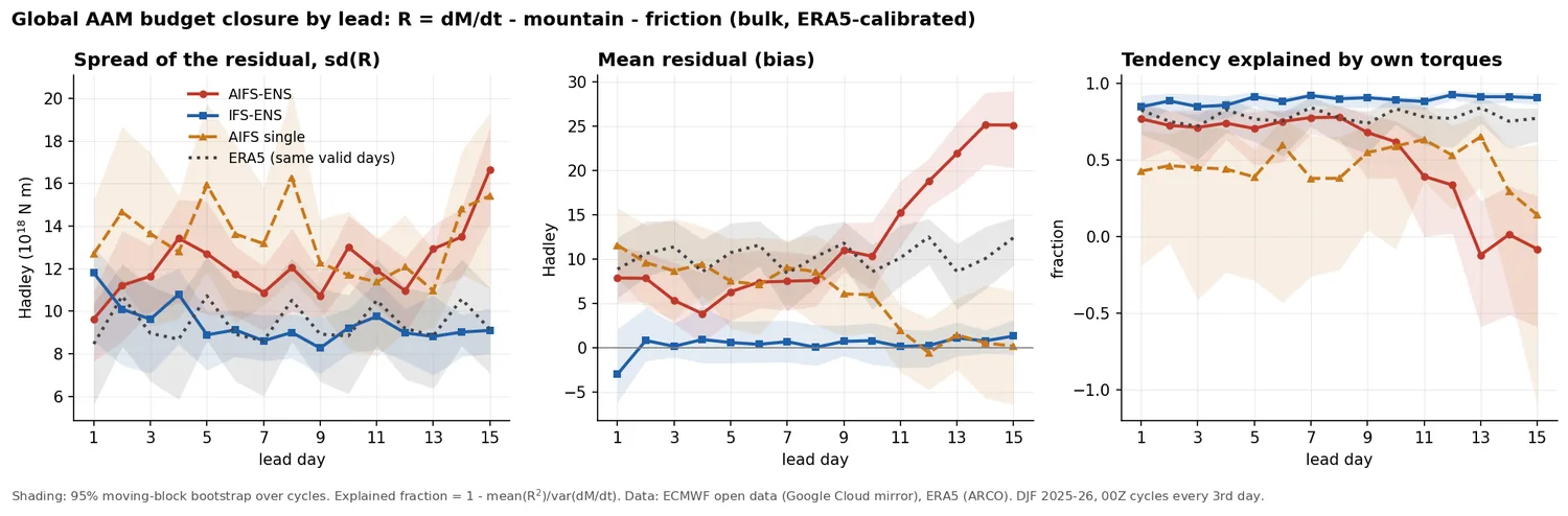
- No, not as well as the physics model. The atmosphere's angular momentum can only change through torques at the surface: pressure pushing on mountains and the drag of the ground on the wind. In IFS-ENS those torques explain 89% of the forecast's own day-to-day change in angular momentum at every lead. In AIFS-ENS they explain 72% on days 1–10 and only 11% on days 11–15. The gap is statistically significant on 14 of the 15 lead days.
- Three things cause it. AIFS does not conserve the total mass of the atmosphere, which is the largest source of day-to-day scatter. It carries a steady excess of a few Hadley on days 1–8, a value close to the reanalysis it learned from. And in week 2 it develops a pressure pattern across the Andes that should brake the winds, while its winds do not respond.
- It does not make the forecasts worse where we could measure. AIFS-ENS's angular momentum is at least as close to ERA5 as IFS-ENS's, and its 500 hPa height error is statistically the same. The inconsistency matters for anything that reads the mechanism: torque-based angular momentum forecasts and attributing a jet change to a mountain torque. It matters most past day 10.
Why the question
About the Earth's axis, the atmosphere's angular momentum $M$ (the winds plus the mass carried round by the rotating Earth) obeys
$$\frac{dM}{dt} = T_{\text{mountain}} + T_{\text{friction}} + T_{\text{gravity-wave drag}}$$
(see the angular momentum and mountain torque explainers). In a physics model this budget is built in: the dynamics conserve momentum up to numerical error, and each surface stress is calculated. A data-driven model such as AIFS has no conservation law. It learns to predict the next state from the last, and nothing ties the change in its winds to the pressure it places against the mountains or to the drag implied by its own surface winds. A budget test asks whether each forecast is consistent with itself, separately from whether it is accurate.
What was done
- Forecasts: ECMWF open data, 30 cycles at 00Z, every third day from 1 December 2025 to 26 February 2026, days 1–15. No cycle or step was missing. Runs per cycle: AIFS-ENS member 0 and perturbed members 1–3, IFS-ENS control and perturbed members 1–3, and the deterministic AIFS single. In the open data the IFS high-resolution forecast is bit-identical to the IFS-ENS control, so the control stands in for it. Fields: surface pressure and 10 m wind every 6 hours (plus IFS's own accumulated surface stress), and zonal and meridional wind on the 13 published pressure levels (1000–50 hPa) every 24 hours. Each model's own orography is used.
- Reference: ERA5 for 1 December 2025 to 16 March 2026, hourly surface fields with its turbulent and gravity-wave surface stresses, and winds on all 37 levels.
- Budget: lead day $k$ is the 24-hour window ending at hour $24k$. The change in $M$ across the window is compared with the torques averaged over it at 6-hourly steps, which cancels the daily and twice-daily pressure tides exactly. The hemispheric budgets also subtract the angular momentum carried across the equator.
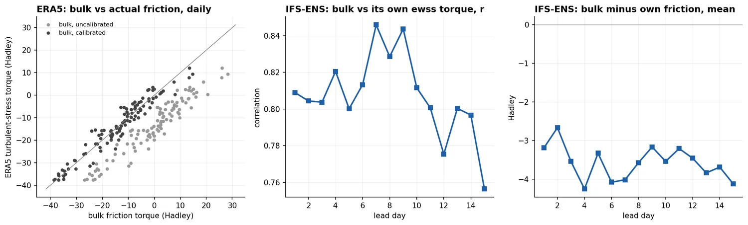
- Friction: AIFS publishes no surface stress, so every model gets the same bulk estimate, $\tau = C_d\,\rho\,|V_{10}|\,u_{10}$, with the site's per-cell drag coefficient, recalibrated over land and sea against ERA5's own stress for this winter (cross-validated r = 0.94, RMSE 4.7 Hadley). Gravity-wave drag is not published for any forecast and stays in the residual. 1 Hadley = 1018 N m.
- Statistics: moving-block bootstrap over cycles (blocks of three consecutive cycles, 2,000 resamples), with model differences paired on the same cycles. "Significant" means two-sided p < 0.05 at that lead day. Every comparison below says which lead days pass, and those that do not are marked n.s.
Results
The global budget
| days 1–5 | days 6–10 | days 11–15 | |
|---|---|---|---|
| Explained fraction | |||
| AIFS-ENS | 0.73 | 0.72 | 0.11 |
| IFS-ENS | 0.87 | 0.90 | 0.91 |
| AIFS single | 0.43 | 0.50 | 0.45 |
| ERA5, same days | 0.78 | 0.79 | 0.78 |
| AIFS-ENS minus IFS-ENS | -0.19 (4 of 5 days) | -0.22 (5 of 5 days) | -0.87 (5 of 5 days) |
| Residual spread, sd (Hadley) | |||
| AIFS-ENS | 11.7 | 11.7 | 13.2 |
| IFS-ENS | 10.2 | 8.8 | 9.1 |
| AIFS single | 13.9 | 13.4 | 12.9 |
| ERA5, same days | 9.5 | 9.2 | 9.7 |
| AIFS-ENS minus IFS-ENS | +1.9 (3 of 5 days) | +2.7 (5 of 5 days) | +3.9 (3 of 5 days) |
| Mean residual (Hadley) | |||
| AIFS-ENS | +6.3 | +8.8 | +21.3 |
| IFS-ENS | -0.1 | +0.6 | +0.7 |
| AIFS single | +9.4 | +7.4 | +0.7 |
| ERA5, same days | +10.1 | +10.1 | +10.8 |
| AIFS-ENS minus IFS-ENS | +6.2 (4 of 5 days) | +8.3 (5 of 5 days) | +20.4 (5 of 5 days) |
Global residual averaged over each band of lead days. Model rows are descriptive. The "AIFS-ENS minus IFS-ENS" rows give the mean difference and the number of lead days in the band where it is significant, or n.s. where no lead day is.
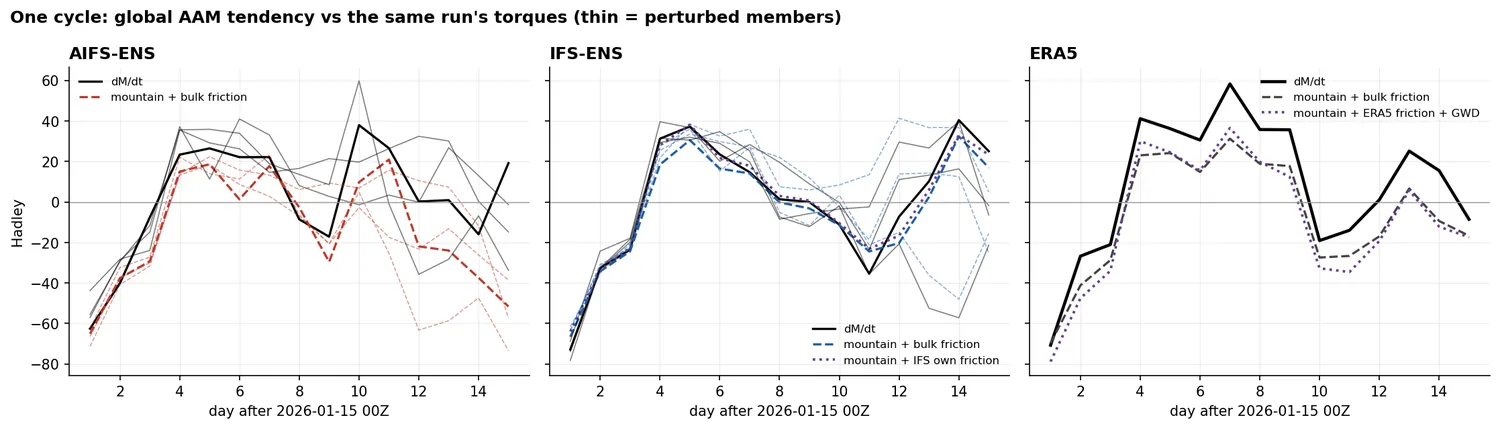
- IFS-ENS closes its budget. With the shared bulk friction its residual averages about zero, and the explained fraction is above ERA5's at 11 of 15 lead days (significant). With IFS's own surface stress the residual falls to 5.4 Hadley spread and -3.0 Hadley mean on days 2–15. That is about the size of the missing gravity-wave drag (ERA5: -5.2 ± 2.2) plus the error from sampling only 13 levels.
- AIFS-ENS closes less well. Its explained fraction is significantly lower than IFS-ENS's on 14 of 15 days (all except day 1), and its residual spread is significantly larger on 11 of 15. Against ERA5 itself, AIFS-ENS is not significantly different on days 1–5 and differs on only one day of days 6–10. It falls well below on all of days 11–15.
- AIFS single explains about 46% of its tendency at every lead, significantly below IFS-ENS on all 15 days. Its residual is no larger than AIFS-ENS's, but its own tendency is smoother, so the same residual is a larger share.
By hemisphere
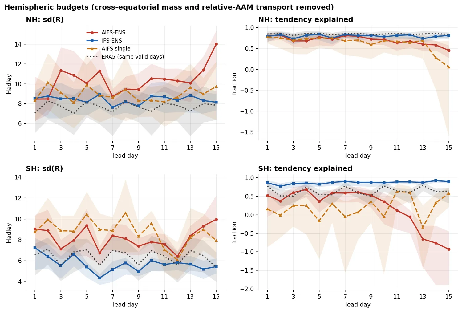
| AIFS-ENS minus IFS-ENS | days 1–5 | days 6–10 | days 11–15 |
|---|---|---|---|
| NH: explained fraction | -0.07 (1 of 5 days) | -0.05 (1 of 5 days) | -0.22 (4 of 5 days) |
| NH: spread (Hadley) | +1.6 (2 of 5 days) | +1.7 (4 of 5 days) | +2.5 (2 of 5 days) |
| SH: explained fraction | -0.38 (5 of 5 days) | -0.42 (5 of 5 days) | -1.55 (5 of 5 days) |
| SH: spread (Hadley) | +2.3 (4 of 5 days) | +2.5 (5 of 5 days) | +2.7 (4 of 5 days) |
After removing the cross-equatorial transport. The deficit is mainly a Southern Hemisphere one.
Cause 1: the total mass of the atmosphere drifts
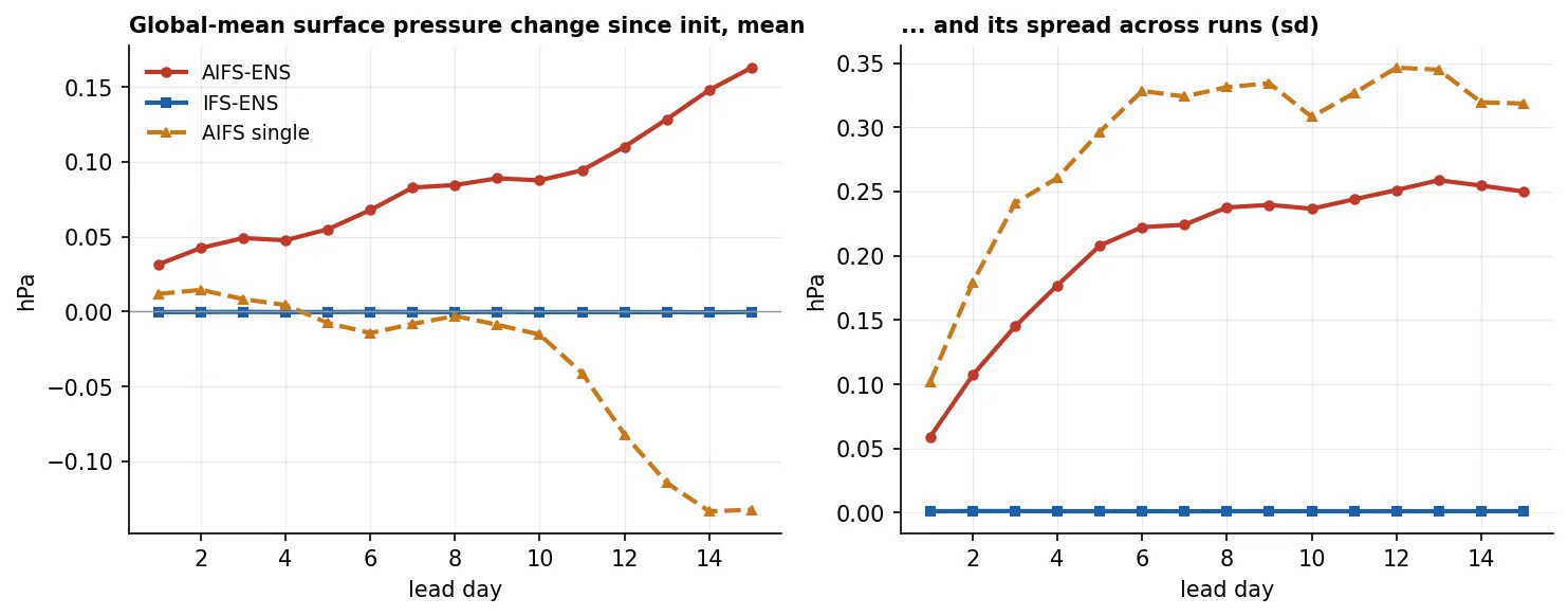
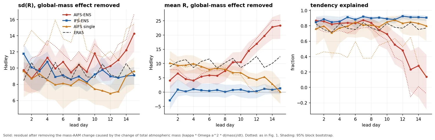
AIFS predicts surface pressure freely, and the global mean wanders: by day 10 the run-to-run spread of the global-mean surface pressure is 0.24 hPa in AIFS-ENS and 0.31 hPa in AIFS single. IFS holds it at 0.00 hPa because it applies a global mass fixer. Air that appears or disappears changes the mass part of the angular momentum with no torque to account for it. Removing that effect brings AIFS-ENS's residual spread down to IFS-ENS's on days 2–9, with no significant difference on any of those days (p ≥ 0.15). Mass non-conservation is therefore the main source of the extra scatter. AIFS single improves to about 0.8 explained but stays significantly below IFS-ENS at most leads.
Cause 2: a steady excess on days 1–8
Even after the mass correction, AIFS-ENS's angular momentum rises by +4 to +7 Hadley a day more than its torques allow, significantly more than IFS-ENS's near-zero. ERA5, the reanalysis AIFS was trained on, shows a similar excess (+10 Hadley on the same days). This is expected in a reanalysis, because assimilating observations adds momentum that no torque supplies; Veerman and van Heerwaarden (2019) found the same in ERA-20C. One reading is that AIFS has learned the analysed evolution, observation increments included, rather than a closed physical budget. That is a hypothesis; it was not tested here.
Cause 3: the Andes in week 2
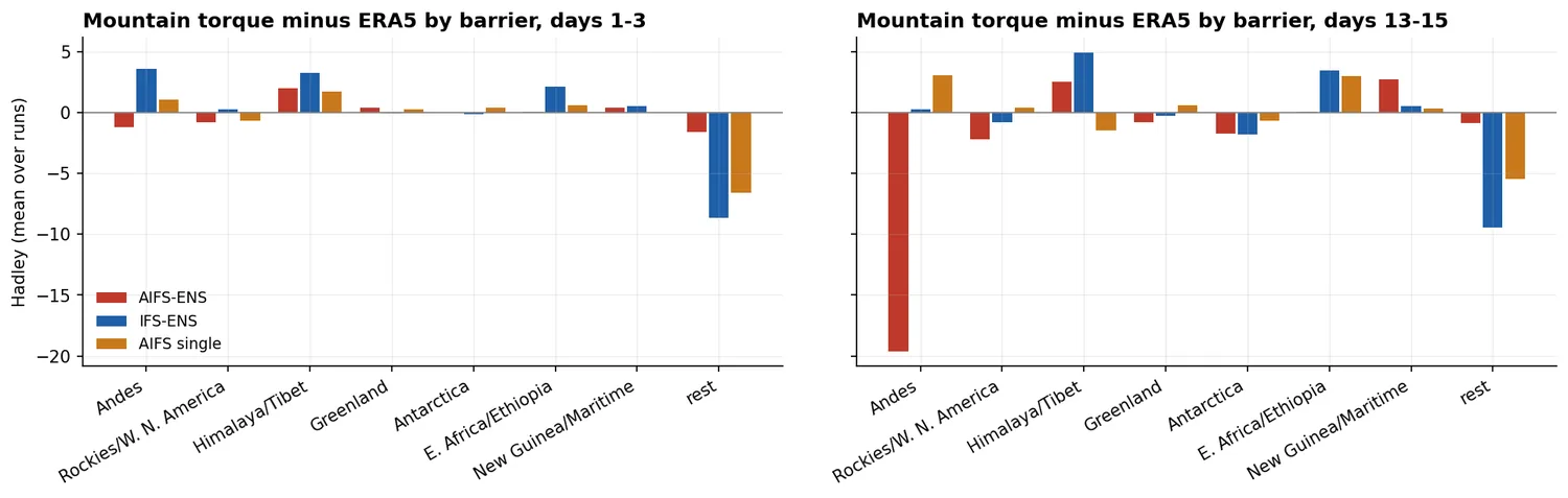
On days 13–15 AIFS-ENS's global mountain torque is -19 Hadley below ERA5's on the same days (95% interval -27 to -11, significant). In the Southern Hemisphere it is -16 (95% interval -22 to -11, significant). For IFS-ENS (-3) and AIFS single (-0) the difference is not significant. Split by mountain range, -20 of the -20 Hadley sits over the Andes. AIFS-ENS builds too strong a high-to-the-west, low-to-the-east pressure contrast across the range, a pattern that should brake the westerlies. Its angular momentum change meanwhile stays unbiased against ERA5, so the torque has no effect on its own winds. The per-range split is descriptive; only the global and hemispheric values were tested.
Does it matter for accuracy?
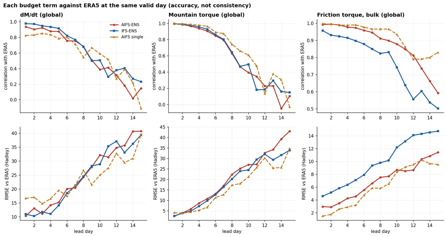
- Angular momentum error: AIFS-ENS's relative angular momentum is closer to ERA5 than IFS-ENS's at every lead day, significantly so at day 5 and day 15. At day 10 the difference (0.40 against 0.50 ×1025 kg m² s⁻¹) is n.s. (p = 0.13). IFS-ENS loses angular momentum steadily (-0.31 ×1025 by day 15) while closing its own budget almost exactly.
- 500 hPa height (20–90°N, RMSE): 112 m for AIFS-ENS against 115 m for IFS-ENS at day 10. The difference is n.s. at days 5, 10 and 15.
- Run by run: a run that closes its budget worse does not have a larger day-10 z500 error. The correlation is n.s. for every model. The one significant link is in angular momentum itself: within a cycle, the AIFS-ENS member with the larger unexplained change by day 10 has the larger total angular momentum error (r = 0.35, 95% interval 0.18 to 0.50). The same link is n.s. for IFS-ENS.
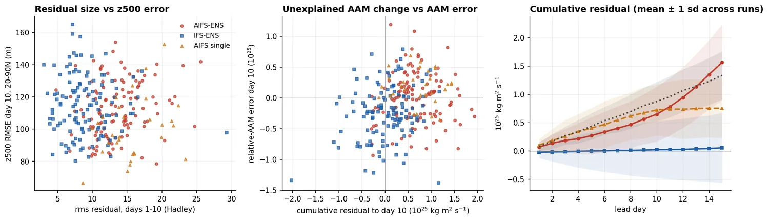
The inconsistency does not show up in headline scores, because the model has learned the analysed evolution of the angular momentum well. It matters for products that read the mechanism, such as this site's torque budget, which is computed from AIFS-ENS. For those, an AIFS-ENS torque past about day 10 is not a cause of its angular momentum change in the way an IFS torque is. The largest contributor, mass drift, is also the most fixable: global mass constraints of the kind Sha et al. (2025) added to another AI model would remove it.
Caveats
- One winter (December–February 2025–26), 30 cycles and four members per ensemble. The Southern Hemisphere and Andes results may depend on the season or on the model version; AIFS-ENS has been upgraded since.
- Only the 13 published pressure levels (1000–50 hPa) were available, the 10 hPa level reaching open data only in mid-2026. For AIFS these are the model's own levels. For IFS they are a subsample, which costs about 5 Hadley of noise (measured in ERA5).
- Friction is a calibrated bulk estimate for every model and adds about 7–8 Hadley of noise to every residual. Against IFS's own stress it behaves the same at every lead (Figure 9).
- Gravity-wave drag is not available from either forecast and stays in the residual. ERA5 puts it at about −5 Hadley this winter, too small and too steady to explain the difference between the models.
- The idea that AIFS reproduces the reanalysis's observation increments is an untested hypothesis.
- The mass correction assumes the spurious air is spread like the real air. It is a diagnostic split, not an exact one.
- A literature search found no earlier angular momentum budget test of an AI weather model. That is a search result, not proof that none exists.
- ERA5 is the reference for accuracy, and it is itself an analysis made with the IFS.
The reference: a reanalysis does not close either
| ERA5, 105 days | mean | sd | explained |
|---|---|---|---|
| bulk friction, 13 levels (as for the forecasts) | +10.5 | 9.3 | 0.79 |
| ERA5's own turbulent stress, 13 levels | +10.5 | 8.1 | 0.81 |
| + ERA5 gravity-wave drag | +15.6 | 7.4 | 0.68 |
| + all 37 levels, hourly mountain torque | +15.7 | 5.3 | 0.69 |
ERA5's own budget over the same winter, in Hadley; the spread of its daily tendency is 31.
ERA5 explains about 80% of its daily change but runs a steady +10 to +16 Hadley excess, which adding gravity-wave drag makes larger. Huang, Sardeshmukh and Weickmann (1999) found the same kind of imbalance in the NCEP reanalysis: total torques about 10 Hadley too low for the observed change, which is the same sign and size as the excess here.
References
- Huang, H.-P., P. D. Sardeshmukh and K. M. Weickmann, 1999: The balance of global angular momentum in a long-term atmospheric data set. J. Geophys. Res., 104, 2031–2040. doi:10.1029/1998JD200068
- Veerman, M. A., and C. C. van Heerwaarden, 2019: Trends in and closure of the atmospheric angular momentum budget in the 20th century in ERA-20C. Q. J. R. Meteorol. Soc., 145, 2990–3003. doi:10.1002/qj.3600
- Hersbach, H., and co-authors, 2020: The ERA5 global reanalysis. Q. J. R. Meteorol. Soc., 146, 1999–2049. doi:10.1002/qj.3803
- Egger, J., K. Weickmann and K.-P. Hoinka, 2007: Angular momentum in the global atmospheric circulation. Rev. Geophys., 45, RG4007. doi:10.1029/2006RG000213
- Bell, M. J., R. Hide and G. Sakellarides, 1991: Atmospheric angular momentum forecasts as novel tests of global numerical weather prediction models. Phil. Trans. R. Soc. A, 334, 55–92. doi:10.1098/rsta.1991.0003
- Toniazzo, T., and co-authors, 2020: Enforcing conservation of axial angular momentum in the atmospheric general circulation model CAM6. Geosci. Model Dev., 13, 685–705.
- Lang, S., and co-authors, 2024: AIFS – ECMWF's data-driven forecasting system. arXiv:2406.01465; and AIFS-CRPS: ensemble forecasting using a model trained with a loss function based on the CRPS. arXiv:2412.15832
- Bonavita, M., 2024: On some limitations of current machine learning weather prediction models. Geophys. Res. Lett., 51. doi:10.1029/2023GL107377
- Sha, Y., J. Schreck, W. Chapman and D. J. Gagne, 2025: Improving AI weather prediction models using global mass and energy conservation schemes. J. Adv. Model. Earth Syst., 17. doi:10.1029/2025MS005138
- Chapman, W. E., J. Schreck and Y. Sha, 2026: Hard conservation correctors can hide a degrading model when training autoregressive emulators. arXiv:2607.18416
Data
Forecasts: ECMWF open data (AIFS-ENS, AIFS single, IFS-ENS), © ECMWF, licensed under CC BY 4.0, fetched from ECMWF's Google Cloud mirror. Reference: ERA5 (Hersbach et al., 2020), Copernicus Climate Change Service (C3S) / ECMWF, via the ARCO-ERA5 store on Google Cloud; contains modified Copernicus Climate Change Service information 2026. Neither ECMWF nor the European Commission is responsible for any use of this information. About 128 GB of forecast fields and 95 GB of ERA5 were read for this study.